| Note on results presented here |
|---|
|
Results presented below are taken from my Master Thesis: Maciej Matyka, "Simulation of incompressible fluid flow phenomena with SIMPLE-MAC method", University of Wroclaw, Poland I am going to defend my master thesis somwhere in the middle of january. So it is first time when those results were published. On an Simulations CD you will find animations presented here. SIMPLE-MAC code will not be published at the moment. If you are interested to get more detailed (numerical) results from my simulations presented here, or calculate something interesting with the SIMPLE-MAC code, just let me know via email. Of course, after my MSc defend, since I need to learn now until middle of january. Wish me good luck on my MSc defend, Maciej Matyka, 2005-01-02  Some people have problems with .mpg anims. Click here to
find .avi versions tested to play under
mplayer windows port. Some people have problems with .mpg anims. Click here to
find .avi versions tested to play under
mplayer windows port.
|
| Name | Picture | Animation | Description |
|---|---|---|---|
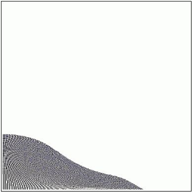
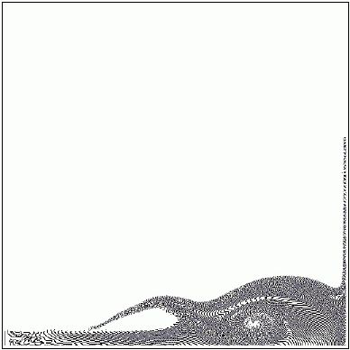
| Broken-dam |
 t=0.0 t=0.0
 t=1.6 t=1.6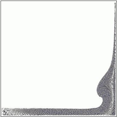 t=4.8 t=4.8
 t=6.4 t=6.4
|
anim1 (~3.5 Mb) |
Well known Broken-dam problem has been solved with SIMPLE-MAC free surface solver. I've
used this case as a one of code validation test and results were tested with Deborah Graves paper published in 2004.
I've also compared my results with an experimental datas and I've got really good agreement.
Simulation presented in an animation (link on the left) has been prepared with SIMPLE-MAC code and following initial/physics conditions have been applied: - kinematic viscosity: 1*10^{-3} kg/m/s - fluid density: 1000 kg/m^3 - grid resolution NX: 80 - grid resolution NY: 80 - maximum delta time DT = 0.01 - gravity GY = -9.8 m/s Visualization: marker particles (each pixel = one marker particle). |
| 90 degrees knee |
 Re=50.0 Re=50.0
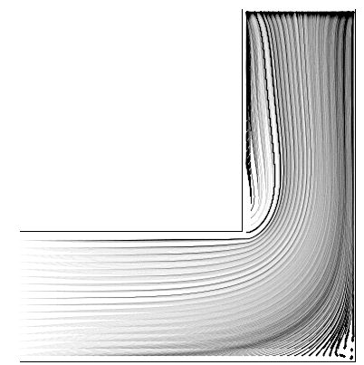 Re=100. Re=100.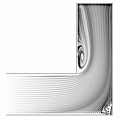 Re=200. Re=200.
 Re=300. Re=300.
|
anim1 (~1.96 Mb) anim2 (~19.0 Mb) |
I have tested also a non-surface fluid flow trough 90 degrees courved tunnel for couple different
Reynolds number.
Simulation presented in an animation (link on the left) has been prepared with SIMPLE-MAC code and following initial/physics conditions have been applied: - grid resolution NX: 120 - grid resolution NY: 120 - maximum delta time DT = 0.01 - gravity GY = 0.0 m/s - Reynolds number Re: 200 Visualization: anim 1 - streamlines and velocity field colort (red - x velocity, green - y velocity), anim 2 - marker particles (each pixel = one marker particle). |
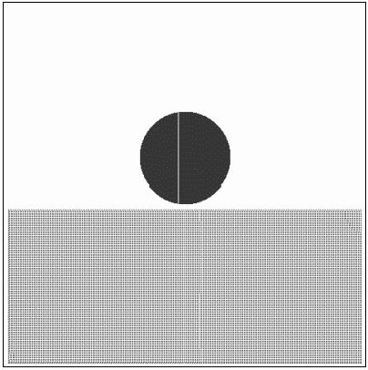
| Liquid Drop on a flat plate |
 t=0.00  t=6.00 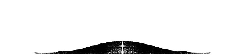 t=14.0  t=18.0 |
anim1 (~0.8 Mb) |
First attempt to splashing drop problem - the case of drop falling onto a flat plate. This case has been
simulated for comparison of the simulation with an existing experimental datas and calculations done by
Harlow and Shannon from Los Alamos University.
Simulation presented in an animation (link on the left) has been prepared with SIMPLE-MAC code and following initial/physics conditions have been applied: - inviscid fluid - init drop velocity VY: -1.0 - grid resolution NX: 80 - grid resolution NY: 30 - drop radius R: 10 - maximum delta time DT = 0.005 - gravity GY = -10.0 Visualization: marker particles (each pixel = one marker particle). |
| The Splash of Liquid Drop |
 t=0.0 t=0.0
 t=4.5 t=4.5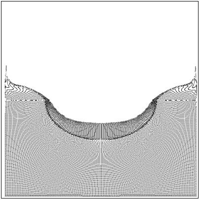 t=9.0 t=9.0
 t=22.5 t=22.5
|
anim1 (~2.24 Mb) |
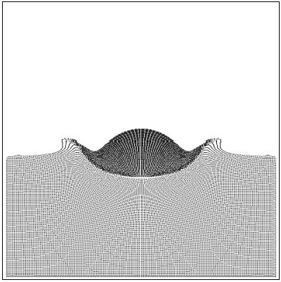
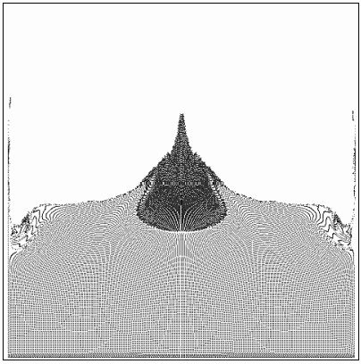
One of my favorite free surface fluid problem - the splash of a liquid drop into a deep pool. I was trying
to obtain results as much close to results obtained by Harlow and Shannon (classic MAC marker-and-cell method) in late 60'
with my SIMPLE-MAC code. I've got really nice results, but I did not obtain one of the most
important effects - seperation of the fluid material in the last stage of simulation (from the top of Worthington jet).
In the thesis I was also trying to find explanation for this.
Simulation presented in an animation (link on the left) has been prepared with SIMPLE-MAC code and following initial/physics conditions have been applied: - inviscid fluid - init drop velocity VY: -1.0 - grid resolution NX: 80 - grid resolution NY: 80 - drop radius R: 10 - maximum delta time DT = 0.005 - gravity GY = -10.0 Visualization: marker particles (each pixel = one marker particle). |
| Staggered tubes |
 |
anim1 (~13.0 Mb) anim2 (~14.0 Mb) |
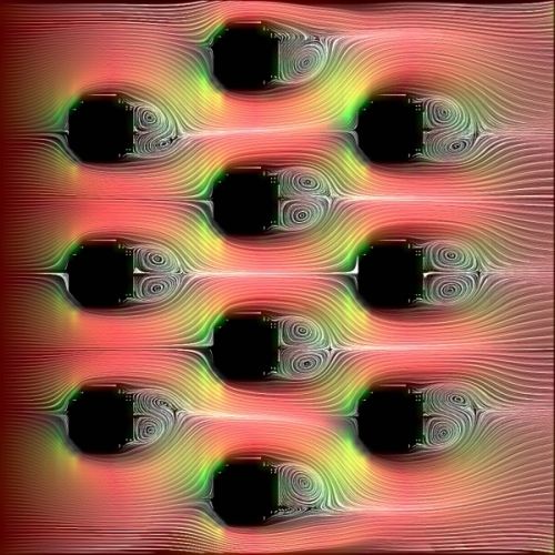
An example of staggered tube bundles flow for Re=149.
Simulation presented in an animation r6-pekrur149_streaklines.mpg (link on the left) has been prepared with SIMPLE-MAC code and following initial/physics conditions have been applied: - viscous fluid - inflow velocity (left) U0: 1.0 - grid resolution NX: 160 - grid resolution NY: 160 - maximum delta time DT = 0.002 - gravity GY = 0.0 Visualization: streaklines. |
| von Karman Vortex Street |
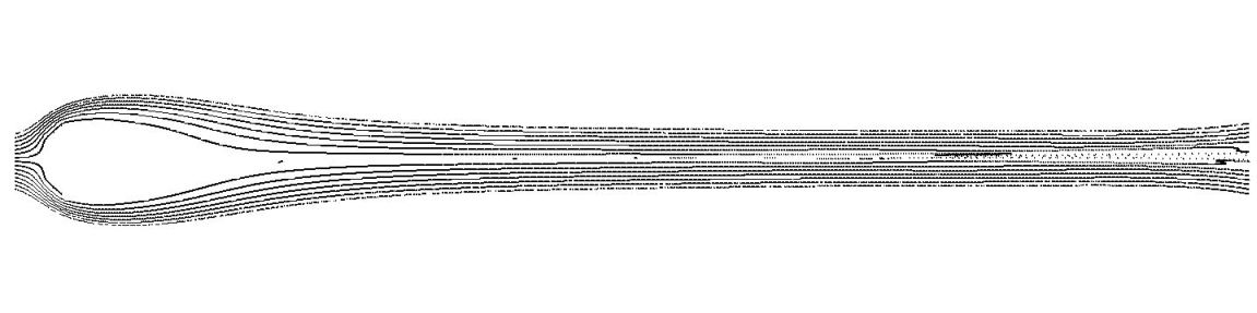 Re=50.00 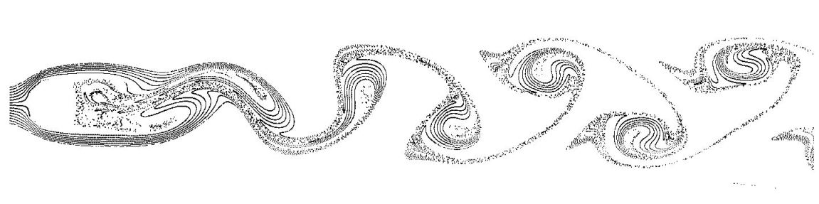 Re=75.00 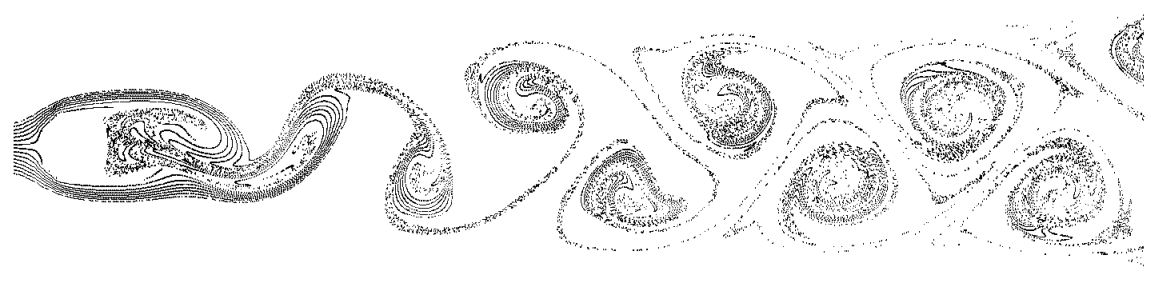 Re=120.0 |
anim1 (~1.0 Mb) anim2 (~2.6 Mb) anim3 (~6.6 Mb) | Classic von Karman Vortex Street for three different Reynolds numbers calculated with
SIMPLE-MAC code.
Visualization: streaklines (not streamlines!). |
| von Karman Vortex Street |
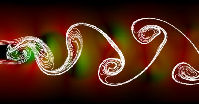 Re=220.0 |
anim4 (!) (~24.1 Mb) |
Classic von Karman Vortex Street has been also obtained on very dense grid
I've did
this simulation because of beauty of vortex street pictures.
Simulation presented in an animation r6-vkRe200_color.mpg (link on the left) has been prepared with SIMPLE-MAC code and following initial/physics conditions have been applied: - viscous fluid - init velocity profile (left wall) ~x^2 (max u=1.4 in the cylinder center) - grid resolution NX: 200 - grid resolution NY: 70 - maximum delta time DT = 0.001 - gravity GY = 0.0 - Re=200 Visualization: streaklines and velocity color field (x velocity intensity - red, y velocity intensity - green). |